Diffusion Model 是如何制作的?
- 生成图片的第一步: 生成 一个都是杂讯的图片,生成图片的大小和目标图片大小一致。
- 然后进行 denoise,就是过滤掉先前图片中的部分杂讯
- 不断进行 denoise,最后得到一张清晰的图片
- 每一步 denoise 都有一个编号,越之后的步骤的 denoise 的编号越小

从杂讯到图片的过程称为 reverse process。
跟雕塑一样
denoise 的模型,除了需要输入一张图片之外,还要一个代表当前图片 noise 的程度的输入。

Denoise 模组内部实际做的事情
denoise 模组内部有一个 noise predicter,预测图片中的杂讯长什么样,需要输入一张图片和图片的 noise 程度,然后输出一张输入图片的杂讯,减去输入图片,达到 denoise 的效果

直接产生一张更清晰的图片比产生一种 noise 图片更难,所以现在大部分模型都会选择先产生一张 noise 的图片
如何训练 noise predictor?

- 对图片不断加 noise
把某次加noise后的图片作为输入,对应的 noise 就是它的输出

Text-to-Image
- 训练 文字-图片生成模型,需要文字-图片成对的资料
- 大部分图片来源于 laion(网站?)
- 在训练 denoise model 的时候,加入 文字

Stable Diffusion
Framework
三个组成部分:
- Text Encoder:文字叙述 编程 一个一个的向量
Generation Model:输入一个杂讯 和 文字的decoder译码结果,然后产生一个中间产物
- 中间产物,是图片的压缩版本,可以是图片模糊的版本,也可以根本看不出来
- Decoder:图片压缩版本还原成最终图片
三个组成部分是分开训练的,然后把他们组合起来的

Stable Diffusion

① 文字的译码器 Text Encoder
② 生成模型 generation model
③ 解码器 decoder
Fréchet Inception Distance(FID)
- 现有一个 CNN model 和 影像分类的模型
- 把真实图片和生成图片输入 CNN 模型中,产生 representation
- 然后比较两组的 representation
- 用来衡量图片生成好坏的模型
- 需要大量的样本支撑
- FID 是把图片当成 Gaussian 高斯图片,然后计算图片之间的距离
- 真实图片和生成图片之间的距离越小越好

Decoder
- 训练 decoder 的时候不需要 文字 和 图片 的成对资料
- 如果中间产物为小图,那么 decoder 的训练就是把一张图片的小图作为输入,然后生成大图
如果中间产物是 Latent Representation,就是训练一个 latent encoder,让一张图片输入到latent encoder 中,然后把输出的 latent representation 通过 decoder 还原图片,两张图片越接近越好。就这样训练 decoder,训练完成之后就可以把 decoder 单独拿出来去解码 latent representation。

如果输入图片是 $H\times W\times 3$ (H: height, W:width, 3: RGB),那么输出图片就可以认为是 $h\times w \times c$ ,它可以是人类看不懂的图片
Generation Model
训练 Noise predicter:
- 用一张图片和一个 encoder 产生一张 latent representation,再用杂讯加在 latent representation,不断加杂讯。
Noise Predicter的输入:
- 加入杂讯后的 latent representation
- step 编号的输入(代表和原来 latent representation 之间差距)
- 文字的输入(文字是用一排向量表示,也是 latent representation)

Diffusion Model 背后的数学原理
基本概念
Forward Process
就是给一张图片,然后不断添加 noise
Reverse Process
给一个全 noise 的 图片,每次 denoise,图片都会一点点浮现出来,到最后呈现的是完整的图片
VAE vs. Diffusion Model
VAE
[photo] => Encoder => Latent Representation => Decoder => [photo]
Diffusion
[photo] => Add noise(固定好的,人设计的,不需要训练) => [只有杂讯的image] => denoise => [photo]

Denoising Diffusion Probabilistic Models

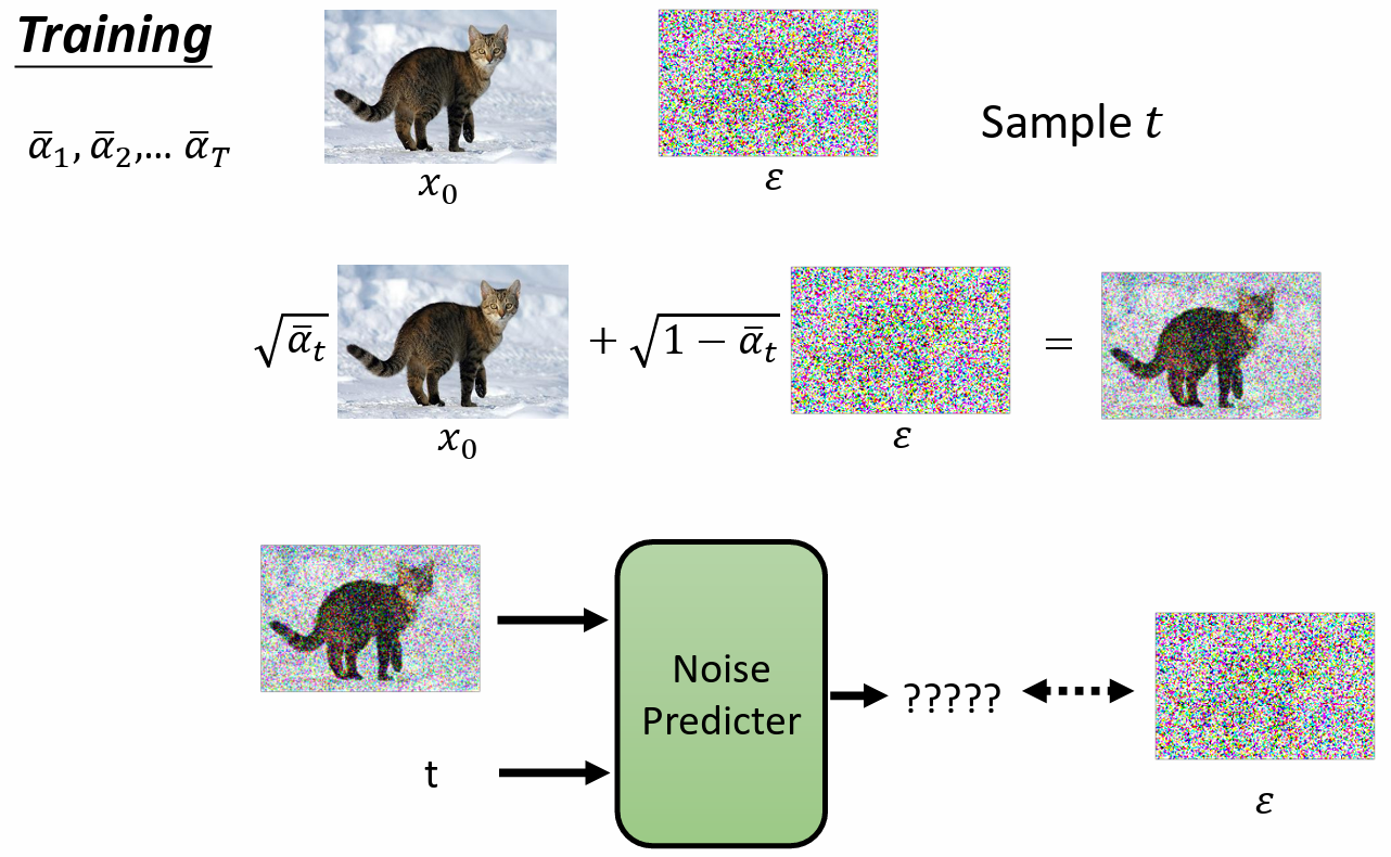
Training
- 1: repeat 重复
- 2:sample 一张 image $x_0$,$x_0$ 代表干净的图
- 3:从一个较大数的范围内 sample 一个数字 $t$ 出来
- 4:$\epsilon$ 是从 normal distribution 中训练出来的,sample a noise
5:采取梯度下降法 $ \nabla_{\theta} \Vert \epsilon - \epsilon_{\theta}(\sqrt{\bar{\alpha}_t}x_0+\sqrt{1-\bar{\alpha}_t}\epsilon, t)\Vert$
- $\epsilon$ :target noise
- $\epsilon_{\theta}$:noise predictor
- t 越大,$\bar{\alpha}_t$ 越小,离 $x_0$ 越远,离 target noise $\epsilon$ 越近
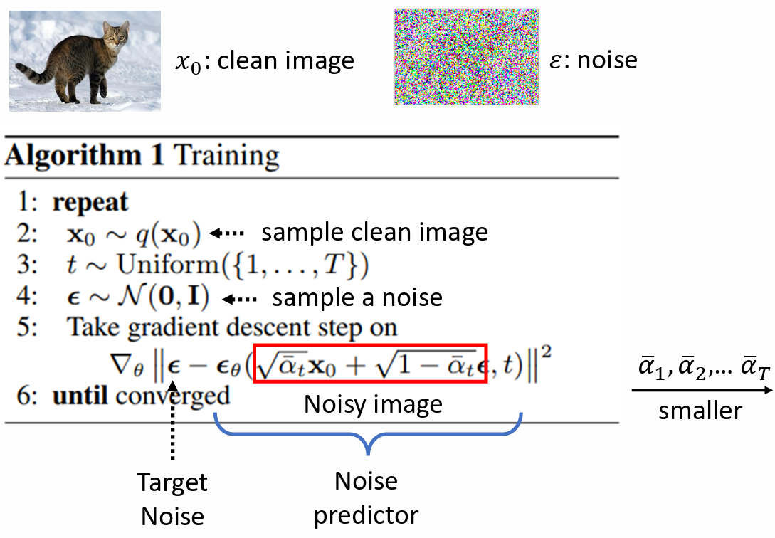

实际上:
- 干净图直接混入一个噪音,通过 $\bar\alpha_t$ 直接决定噪音的大小,得到一个有噪音的图
- 训练的时候,把有噪音的图 和 t 当作输入,直接预测 混入的 噪音
Sampling
产生图片的过程:
- 一开始,sample 一个全是 noise 的图 $x_T$
运行 T 次,t = T, ..., 1 do
- 再 sample 一次 noise $\boldsymbol{z}$
$\boldsymbol{x}_{t-1} = \cfrac{1}{\sqrt{\alpha}_t}\big(\boldsymbol{x}_t - \cfrac{1-\alpha_t}{\sqrt{1-\bar\alpha_t}}\epsilon_{\theta}(\boldsymbol{x}_t, t)\big) + \sigma_t \boldsymbol{z}$
- x_t 是上一个步骤产生出来的图
- $\epsilon_{\theta}$ 是 noise predicter 输出的 noise

影像生成模型本质上的共同目标
- Gaussian distribution:正态分布
- 在 input 的地方有一个简单的 distribution,通常是 Gaussian distribution(正态分布)
- 从 input 的地方 sample 一个东西出来,通常是 vector,然后把这个 vector 放在 network 里面去, $G(z) = x$ ,z 表示输入,x 就是一张图片
- 每次从 input 的地方 sample 一个 vector 出来,通过 network 就变成一张图片。
- 就算输入是非常简单的 Gaussian distribution ,通过 network 转换,输出会变成一张张图片,这些图片会组合成非常复杂的 distribution。
我们期待的事情是,我们找到一个 network,这个 network 应该做到的事情是跟真正的图片的 distribution 和真正图片所形成的 distribution 越接近越好。

Maximum Likelihood Estimation
什么叫做越接近越好?
- 大部分利用 Maximum Likelihood Estimation 判断
假设 network 的参数为 $\theta$ ,然后根据 $\theta$ 产生的 distribution 表示为 $P_\theta(x)$,真正的 distribution 表示为 $P_{data}(x)$ (Maximum Likelihood Estimation)
首先从 $P_{data}(x)$ 中 sample 一堆 image $\{x^1, x^2, ..., x^m\}$ 出来
- $P_{data}(x)$ 是所有可能搜集到的训练资料
- 假设我们能够计算 $P_\theta(x^i)$
- 我们要找$\theta$ 是 $\theta^* = arg \max_\theta\prod^m_{i=1}P_\theta(x^i)$
使得产生 $x^1, x^2, \cdots, x^m$ 这些图片的概率的乘积最大
Sample $\{x^1, x^2, \dots, x^m\}$ from $P_{data}(x)$
$$ \begin{align} \theta^* &= arg\max_\theta\prod^m_{i=1}P_\theta(x^i) = arg\max_\theta\log\prod^m_{i=1}P_\theta(x^i)\\ &= arg\max_\theta\sum^m_{i=1}\log P_\theta(x^i) \approx arg\max_\theta E_{x\sim P_{data}}[\log P_\theta (x)] \\ &= arg\max_\theta \int_x P_{data}(x)\log P_\theta (x) \mathrm{dx} - \int_x P_{data}(x)\log P_{data} (x)\mathrm{dx}\\ &= arg\max_\theta \int_x P_{data}(x)\log \cfrac{P_\theta (x)}{P_{data} (x)} \mathrm{dx} \\ &= arg \min_\theta KL(P_{data}\Vert P_\theta) \end{align} $$
KL Divergence 计算两个 distribution 的差异程度
$KL(P_{data}\Vert P_\theta)$ :Difference between $P_{data}$ and $P_\theta$
越大,差异越大
- Maximum Likelihood = Minimize KL Divergence

VAE
Compute $P_\theta(x)$
- z => network => G(z) = x (arg = $\theta$) => 计算 $P_\theta(x)$
VAE 假设 输入 z,输出 G(z),G(z) 代表 Mean of Gaussian
所以 $P_\theta(x|z) \propto \exp(-\Vert G(z) - x\Vert_2)$
- $\Vert G(z) - x\Vert_2$ 表示 $G(z)$ 和输入数据 $x$ 之间的欧氏距离
Lower bound of $\log P(x)$
$$ \begin{align} \log P_\theta(x) & = \int_z q(z|x) \log P(x) \mathrm{dz}\\ &= \int_z q(z|x) \log\bigg(\cfrac{P(z,x)}{P(z|x)}\bigg)\mathrm{dz} = \int_z q(z|x) \log\bigg(\cfrac{P(z,x)}{q(z|x)}\cfrac{q(z|x)}{P(z|x)}\bigg)\mathrm{dz}\\ &= \int_z q(z|x) \log\bigg(\cfrac{P(z,x)}{q(z|x)}\bigg)\mathrm{dz}+\int_z q(z|x) \log\bigg(\cfrac{q(z|x)}{P(z|x)}\bigg)\mathrm{dz}\\ & \geqslant \int_z q(z|x)\log \bigg(\cfrac{P(z,x)}{q(z|x)}\bigg)\mathrm{dz} = \mathrm{E}_{q(z|x)}[\log\bigg(\cfrac{P(z,x)}{q(z|x)}\bigg)] \end{align} $$
- 因为logP(x)与z无关,所以可以提出积分外面,那么积分里面的东西,积完以后就是1,右边跟左边一样,所以 $\log P_\theta(x)$ 与 $q(z|x)$ 无关
- $\int_z q(z|x) \log\bigg(\cfrac{q(z|x)}{P(z|x)}\bigg)\mathrm{dz} = KL(q(z|x)\Vert P(z|x)) \geqslant 0$
- $\log P_\theta(x)$ 的 lower bound 是 $\mathrm{E}_{q(z|x)}[\log\bigg(\cfrac{P(z,x)}{q(z|x)}\bigg)]$
- 如果可以 Maxmize 这个 lower bound,就可以使得 $\log P(x)$ 得到一个较大的值
- 在 VAE 中,$\mathrm{E}_{q(z|x)}$ 就是 Encoder
DDPM
Compute $\log P_\theta(x)$
- 可以把 denoise 的过程想成产生 Gaussian distribution,当输入 $x_t$ 输入 denoise model,就会产生一个 结果 $G(x_t)$ ,把这个 output 的结果想成 Mean of Gaussian。
- 如果 $x_{t-1}$ 和 output 的结果正好一模一样,是几率最大的 case,如果差很远,几率就小很多
$P_\theta(x_0) = \int_{x_1: x_T} P(x_T)P_\theta(x_{T-1}|x_T)...P_\theta(x_{t-1}|x_t)...P_\theta(x_0|x_1) \mathrm{dx_1:x_T}$
对所有可能的 $x_1: x_T$ 做积分

Lower bound of $\log P(X)$
VAE: Maximize $\log P_\theta(x)$ => Maximize $\mathrm{E}_{q(z|x)}[\log \bigg(\cfrac{P(x,z)}{q(z|x)}\bigg)]$
- $q(z|x)$ 是 Encoder
DDPM Maximize $\log P_\theta(x_0)$ => Maximize $\mathrm{E}_{q(x_1:x_T|x_0)}[\log \bigg(\cfrac{P(x_0:x_T)}{q(x_1:x_T|x_0)}\bigg)]$
$q(x_1:x_T|x_0)$ 是 Forward Process(Diffusion Process)
就是加 noise 的过程
- $q(x_1:x_T|x_0) = q(x_1|x_0)q(x_2|x_1)...q(x_T|x_{T-1})$
计算 $q(x_t|x_{t-1})$
- $x_1 = \sqrt{1-\beta_1}x_0 + \sqrt{\beta_1}\ noise1, noise1\sim\mathcal{N}(0,I)$
- $x_2 = \sqrt{1-\beta_2}x_1 + \sqrt{\beta_2}\ noise2, noise2\sim\mathcal{N}(0,I)$
- noise1 和 noise2 都是从同样的高斯分布 Gaussian distribution 采样 sample 出来,但是这两次 sample 是相互独立
可以把 $x_1$ 代入 $x_2$ 的公式中,得到
$x_2 = \sqrt{1-\beta_2}\sqrt{1-\beta_1}x_0 + \sqrt{1-\beta_2}\sqrt{\beta_1}noise1 + \sqrt{\beta_2}\ noise2$
$noise1,noise2\sim\mathcal{N}(0,I)$
$\sqrt{1-\beta_2}\sqrt{\beta_1}noise1 + \sqrt{\beta_2}\ noise2 = \sqrt{1-(1-\beta_2)(1-\beta_1)}noise$
$noise\sim \mathcal{N}(0, I)$
所以,$x_2 = \sqrt{1-\beta_2}\sqrt{1-\beta_1}x_0 + \sqrt{1-(1-\beta_2)(1-\beta_1)}noise$


- 以此类推,$x_t = \sqrt{1-\beta_1}...\sqrt{1-\beta_t} x_0 + \sqrt{1-(1-\beta_1)...(1-\beta_t)}noise$
$\alpha_t = 1-\beta_t, \bar\alpha_t = \alpha_1\alpha_2...\alpha_t$
则 $x_t = \sqrt{\bar\alpha_t} x_{t_0} + \sqrt{1-\bar\alpha_t} noise$
Lower bound of $\log P(x)$ :
$$ E_{q(x_1|x_0)}[\log P(x_0|x_1)]-KL(q(x_T|x_0)\Vert P(x_T))-\sum^T_{t=2}\mathrm{E}_{q(x_t|x_0)}[KL(q(x_{t-1}|x_t,x_0)\Vert P(x_{t-1}|x_t))] $$
how to maximize $\sum^T_{t=2}\mathrm{E}_{q(x_t|x_0)}[KL(q(x_{t-1}|x_t,x_0)\Vert P(x_{t-1}|x_t))]$
$q(x_{t-1}|x_t, x_0)$ ,从 $x_0$ 做了n次diffusion生成 $x_t$ ,求 $x_{t-1}$ 的分布(中间过程未知)
$$ \begin{align} q(x_{t-1}|x_t, x_0) &= \cfrac{q(x_{t-1}, x_t, x_0)}{q(x_t, x_0)} = \cfrac{q(x_t|x_{t-1})q(x_{t-1}|x_0)q(x_0)}{q(x_t|x_0)q(x_0)} \\&= \cfrac{q(x_t|x_{t-1})q(x_{t-1}|x_0)}{q(x_t|x_0)} \end{align} $$


- 我们不需要把 KL 算出来,我们只需要 minimize KL divergence
- $q(x_{t-1}|x_t, x_0)$ 是固定的高斯分布 Gaussian distribution,和 network 没有关系,mean 是固定的,variance 是固定的。
- $P(x_{t-1}|x_t)$ 是 由 network 决定,它的 variance 是固定的,只考虑 mean,mean 取决于 denoise model


$x_0$ 是先给定的
通过 $x_t = \sqrt{\bar\alpha_t} x_0 + \sqrt{1-\bar\alpha_t}\epsilon$ sample 出 $x_t$


$x_t = \sqrt{\bar\alpha_t} x_0 + \sqrt{1-\bar\alpha_t}\epsilon$ => $\cfrac{x_t-\sqrt{1-\bar\alpha_t}\epsilon}{\sqrt{\bar\alpha_t}} = x_0$


Diffusion Model for Text
- difficulty: 难以在文字这种 description 上加 noise
Solution:
不在文字上加 noise
Noise on latent space

- 不加 Gaussian noise,加其他种类的 noise